library(data.table) # for data wrangling
#if you need to install esemComp
# devtools::install_github("MateusPsi/esemComp")
library(esemComp)

esem_data <- fread("ESEM.dat")
# keep only first occasion and only the indicators
esem_data <- esem_data[V13 == 1, c(1:6)]
# rename variables to x1,x2...
names(esem_data) <- paste0("x", c(1:6)) The esemComp package
A while back I made a post about Exploratory Structural Equation Modeling (ESEM) in R. To be precise, how to do ESEM-within-CFA in R. Since then, I teamed up with Leon T. de Beer to develop esemComp, an R package to facilitate running these models. The package name is due to its main functionality allowing the composition of a model syntax to be run in the prominent SEM package lavaan.
Here I will run the same analysis as in my original post, but with esemComp functions. You’ll see that with the package the analysis gets much more straightforward. Furthermore, I’ll show how to do the analysis with a target rotation matrix for the exploratory factor analysis step, since this is the preferred approach. In this post, I’ll cut right to the chase, if you need a quick introduction to ESEM, check my original post.
We are going to use the toy dataset used in the examples by Morin et al. (2013). It shows the data for 4500 participants in two occasions (3000 in the first, 1500 in the second). The scale is composed of six items, with three items related to a first factor and three to another, also, two of the items have significant cross-loadings. You can download the data here or at the original supplemental material.
Step one: EFA
First, load the data.
      x1    x2    x3    x4    x5    x6
   <num> <num> <num> <num> <num> <num>
1:  0.10  0.30 -0.42 -0.54 -1.79  1.64
2:  1.69  1.95  2.41  2.53  2.53  0.84
3:  0.71 -0.17 -1.25 -0.49 -1.65 -0.48
4:  2.09  0.37 -0.14  1.27  0.67  2.72
5:  0.03 -0.15  1.22  0.06  0.90  1.09
Running the EFA with two factors and the GeominQ rotation in esemComp is actually pretty similar to using the psych package in R:
esem_efa <- esem_efa(esem_data, nfactors =2, fm = 'ml', delta = .5)
esem_efa$loadings
Loadings:
   ML1    ML2
x1  0.827
x2  0.696  0.226
x3  0.525  0.313
x4  0.138  0.762
x5  0.160  0.672
x6         0.554

                 ML1   ML2
SS loadings    1.491 1.489
Proportion Var 0.249 0.248
Cumulative Var 0.249 0.497
If you want to use the approach recommended in some of the ESEM literature, a target rotation matrix, esemComp got you covered. A target rotation matrix is simply a matrix that represents an expected factor structure. The columns are the factors and the rows are the items, each cell is filled with either a zero or a one. In the rotation process, loadings corresponding to zeros are biased to be as close to zero as possible, and loadings corresponding to one are freely estimated.
In R, if we set ones, the values are actually biased toward one, so we use NA to represent free estimation. That is what the target matrix looks like for our toy data:
target_rot <- make_target(6,mainloadings = list(f1 = 1:3, f2 = 4:6))
target_rot
f1 f2
[1,] NA 0
[2,] NA 0
[3,] NA 0
[4,] 0 NA
[5,] 0 NA
[6,] 0 NAThen, we simply use the target rotation to run the EFA:
esem_target_efa <- esem_efa(esem_data, nfactors =2,
                            target = target_rot,
                            fm = 'ml')
esem_target_efa$loadings
Loadings:
   ML1    ML2
x1  0.923 -0.200
x2  0.751  0.103
x3  0.551  0.230
x4         0.781
x5  0.110  0.681
x6 -0.115  0.598

                 ML1   ML2
SS loadings    1.750 1.536
Proportion Var 0.292 0.256
Cumulative Var 0.292 0.548
We can see that the target rotation makes the main loadings a little stronger and the cross-loadings a bit weaker. From here on, if we wanted to keep using the target rotation solution, we would only need to use this solution whenever a EFA object is needed in the next steps. We’ll continue to use the Geomin solution, tough, to be loyal to the orginial post.
Step two: set ESEM model
To compose the syntax of the ESEM-within-CFA model we need to identify a referent for each factor: an item that loads heavily on that factor but lightly on the others. We have a helper function for that in the package:
referents <- find_referents(esem_efa,factor_names = c("f1","f2"))Those referents make sense when we check the loadings from the EFAs.
Now to compose the model syntax to be used in lavaan. All loadings are estimated with the loadings of the EFA as starting points in ESEM-within-CFA, except for the crossloadings of the referent items. Just pass the EFA object and the referents to the syntax composer and voilà!
#make model
esem_model <- syntax_composer(esem_efa, referents)
#print model
writeLines(esem_model)
f1 =~ start(0.827)*x1+
start(0.696)*x2+
start(0.525)*x3+
0.138*x4+
start(0.16)*x5+
start(-0.053)*x6
f2 =~ -0.036*x1+
start(0.226)*x2+
start(0.313)*x3+
start(0.762)*x4+
start(0.672)*x5+
start(0.554)*x6 Step three: fit ESEM model
Finally, we fit the ESEM model to the data.
library(lavaan)
esem_fit <- cfa(esem_model, esem_data, std.lv=T)
summary(esem_fit, fit.measures = T, standardized = T)
lavaan 0.6-19 ended normally after 23 iterations
Estimator ML
Optimization method NLMINB
Number of model parameters 17
Number of observations 3000
Model Test User Model:
Test statistic 3.897
Degrees of freedom 4
P-value (Chi-square) 0.420
Model Test Baseline Model:
Test statistic 6628.732
Degrees of freedom 15
P-value 0.000
User Model versus Baseline Model:
Comparative Fit Index (CFI) 1.000
Tucker-Lewis Index (TLI) 1.000
Loglikelihood and Information Criteria:
Loglikelihood user model (H0) -21698.913
Loglikelihood unrestricted model (H1) -21696.964
Akaike (AIC) 43431.825
Bayesian (BIC) 43533.933
Sample-size adjusted Bayesian (SABIC) 43479.918
Root Mean Square Error of Approximation:
RMSEA 0.000
90 Percent confidence interval - lower 0.000
90 Percent confidence interval - upper 0.027
P-value H_0: RMSEA <= 0.050 1.000
P-value H_0: RMSEA >= 0.080 0.000
Standardized Root Mean Square Residual:
SRMR 0.004
Parameter Estimates:
Standard errors Standard
Information Expected
Information saturated (h1) model Structured
Latent Variables:
Estimate Std.Err z-value P(>|z|)
f1 =~
x1 0.885 0.022 40.638 0.000
x2 0.636 0.022 28.634 0.000
x3 0.526 0.022 24.210 0.000
x4 0.138
x5 0.125 0.020 6.124 0.000
x6 -0.055 0.022 -2.560 0.010
f2 =~
x1 -0.036
x2 0.212 0.023 9.115 0.000
x3 0.323 0.023 13.906 0.000
x4 0.883 0.021 42.265 0.000
x5 0.585 0.020 28.677 0.000
x6 0.473 0.021 22.414 0.000
Std.lv Std.all
0.885 0.827
0.636 0.690
0.526 0.517
0.138 0.120
0.125 0.145
-0.055 -0.065
-0.036 -0.034
0.212 0.230
0.323 0.318
0.883 0.770
0.585 0.679
0.473 0.560
Covariances:
Estimate Std.Err z-value P(>|z|)
f1 ~~
f2 0.448 0.028 16.025 0.000
Std.lv Std.all
0.448 0.448
Variances:
Estimate Std.Err z-value P(>|z|)
.x1 0.390 0.028 13.948 0.000
.x2 0.279 0.014 20.369 0.000
.x3 0.501 0.015 32.595 0.000
.x4 0.407 0.024 16.625 0.000
.x5 0.320 0.013 25.007 0.000
.x6 0.510 0.015 32.923 0.000
f1 1.000
f2 1.000
Std.lv Std.all
0.390 0.340
0.279 0.328
0.501 0.485
0.407 0.309
0.320 0.430
0.510 0.715
1.000 1.000
1.000 1.000Quick figure with semPlot:
library(semPlot)
semPaths(esem_fit,"std")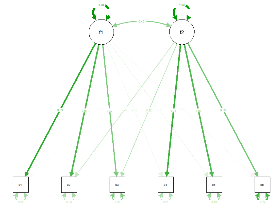
And that is it, ESEM-within-CFA made simple!
References
Morin, Alexandre J. S., Herbert W. Marsh, and Benjamin Nagengast. 2013. “Exploratory Structural Equation Modeling.” In Structural Equation Modeling: A Second Course, 2nd Ed. Quantitative Methods in Education and the Behavioral Sciences: Issues, Research, and Teaching. IAP Information Age Publishing.