library(data.table) # for data wrangling
library(psych) # for EFA

esem_data <- fread("ESEM.dat")
# keep only first occasion and only the indicators
esem_data <- esem_data[V13 == 1, c(1:6)]
# rename variables to x1,x2...
names(esem_data) <- paste0("x", c(1:6)) What is ESEM
Exploratory Structural Equation Modeling is a technique developed by Asparouhov and Muthén (2009) and extended by Marsh. It promises to “integrate the best features of exploratory and confirmatory factor analyses” (Marsh et al. 2014).
Exploratory factor analysis (EFA) is a great tool to investigate the structure of scales in an open and data-driven way. However, it does not allow for extensions of the model to investigate other features, such as measurement invariance and group comparisons, to do that, you need to use a confirmatory model (CFA). But confirmatory models suffer from being overly restrictive, leading to poor fitting to data (for instance, have you ever seen a RMSEA index below .05 as some advise to look for ?).
ESEM comes from the understanding that what impairs CFA fitting is the fixing of all (or most) cross-loadings to zero. The world is messy. But when we fix these cross-loadings to zero what we are doing is entertaining a fiction of a very tidy world where everything fits the theory behind the scale. What ESEM does is try to get the model a little closer to the messiness of the world by allowing all cross-loadings to exist, and, at the same time, do it with a confirmatory technique, which permits model extensions.
Below I show how to do ESEM in R in three steps.
We are going to use a simulated dataset used in the examples by Morin et al. (2013). It shows the data for 4500 participants in two occasions (3000 in the first, 1500 in the second). The scale is composed of six items, with three items related to a first factor and three to another, also, two of the items have significant cross-loadings. You can download the data here or at the original supplemental material.
Step one: EFA
ESEM actually starts with an EFA. The only special thing about it is that we use a GeominQ rotation, which does not emphasize getting rid of cross-loadings. We will use the psych package (Revelle 2020) to do so. First, let’s load the data and keep only the first sample:
      x1    x2    x3    x4    x5    x6
   <num> <num> <num> <num> <num> <num>
1:  0.10  0.30 -0.42 -0.54 -1.79  1.64
2:  1.69  1.95  2.41  2.53  2.53  0.84
3:  0.71 -0.17 -1.25 -0.49 -1.65 -0.48
4:  2.09  0.37 -0.14  1.27  0.67  2.72
5:  0.03 -0.15  1.22  0.06  0.90  1.09
Before we run the EFA with two factors, one point: the GeominQ rotation has a parameter that can affect results. It is usually called epsilon but in this implementation is called delta. One is invited to play with this parameter (usually from .1 to .9) to find the best solution to your specific analysis.1 The EFA is run in the code below, then we check the factor loadings.
esem_efa <- fa(esem_data, nfactors =2,rotate = "geominQ",
               fm = 'ml', delta = .5)
esem_efa$loadings
Loadings:
   ML1    ML2
x1  0.827
x2  0.696  0.226
x3  0.525  0.313
x4  0.138  0.762
x5  0.160  0.672
x6         0.554

                 ML1   ML2
SS loadings    1.491 1.489
Proportion Var 0.249 0.248
Cumulative Var 0.249 0.497
Step two: set ESEM model
Pragmatically, what distinguishes ESEM from EFA and CFA is that we fit a model with the following characteristics:
- A CFA-like model with all cross-loadings and with factor variances fixed
- All cross-loadings set to be estimated with the EFA loadings as starting points, except…
- … that one indicator in each factor is set as an anchor, all its cross-loadings are fixed to be equal to the loading in the original EFA
- The anchors should be indicators with high loading in one factor and low loadings in all the others
We are going to use lavaan (Rosseel 2012) to fit our ESEM model. In lavaan we set starting points for our indicators using the start() modificator, if we write start(.5)*x1 we are saying “use .5 as a starting point for estimating x1 loading”. To set a fixed value we just lose the “start” and parentheses: .5*x1.
It can get very tedious to write up models setting all these parameters, so we are going to set up a function that automates the process. The function inputs will be a data table 2 in long format with columns “item”, “latent” and “value”. The second input is a named vector with the names being each latent variable and values a string with the anchor item for that latent (the item that loads heavily in that latent and poorly to other latents). The function will output a character vector with the model in lavaan syntax.3
Let’s make our inputs. First the data table with item loadings in each factor:
esem_loadings <- data.table(matrix(round(esem_efa$loadings, 2),
                                   nrow = 6, ncol = 2))
names(esem_loadings) <- c("F1","F2")
esem_loadings$item <- paste0("x", c(1:6))
#setDT(esem_loadings)
esem_loadings <- melt(esem_loadings, "item", variable.name = "latent")

esem_loadings
item latent value
<char> <fctr> <num>
1: x1 F1 0.83
2: x2 F1 0.70
3: x3 F1 0.52
4: x4 F1 0.14
5: x5 F1 0.16
6: x6 F1 -0.05
7: x1 F2 -0.04
8: x2 F2 0.23
9: x3 F2 0.31
10: x4 F2 0.76
11: x5 F2 0.67
12: x6 F2 0.55Neat! Now the anchor vector. When we check the loadings, we identify that x1 has high loading in factor 1 and a negligible loading in factor 2, and x2 shows the inverse pattern. So these will be our anchors:
anchors <- c(F1 = "x1", F2 = "x4")Now we let our function munch on the inputs and get our model:
make_esem_model <- function (loadings_dt, anchors){

  # make is_anchor variable
  loadings_dt[, is_anchor := 0]
  for (l in names(anchors)) loadings_dt[latent != l & item == anchors[l], is_anchor := 1]

  # make syntax column per item; syntax is different depending on is_anchor
  loadings_dt[is_anchor == 0, syntax := paste0("start(",value,")*", item)]
  loadings_dt[is_anchor == 1, syntax := paste0(value,"*", item)]

  #Make syntax for each latent variable
   each_syntax <- function (l){
    paste(l, "=~", paste0(loadings_dt[latent == l, syntax], collapse = "+"),"\n")
   }

   # Put all syntaxes together
   paste(sapply(unique(loadings_dt$latent), each_syntax), collapse = " ")
}
#make model
esem_model <- make_esem_model(esem_loadings, anchors)
#print model
writeLines(esem_model)
F1 =~ start(0.83)*x1+start(0.7)*x2+start(0.52)*x3+0.14*x4+start(0.16)*x5+start(-0.05)*x6
F2 =~ -0.04*x1+start(0.23)*x2+start(0.31)*x3+start(0.76)*x4+start(0.67)*x5+start(0.55)*x6 Step three: fit ESEM model
Finally, we fit the ESEM model to the data.
library(lavaan)
library(lavaanPlot)
esem_fit <- cfa(esem_model, esem_data, std.lv=T)
summary(esem_fit, fit.measures = T, standardized = T)
lavaan 0.6-19 ended normally after 23 iterations
Estimator ML
Optimization method NLMINB
Number of model parameters 17
Number of observations 3000
Model Test User Model:
Test statistic 3.897
Degrees of freedom 4
P-value (Chi-square) 0.420
Model Test Baseline Model:
Test statistic 6628.732
Degrees of freedom 15
P-value 0.000
User Model versus Baseline Model:
Comparative Fit Index (CFI) 1.000
Tucker-Lewis Index (TLI) 1.000
Loglikelihood and Information Criteria:
Loglikelihood user model (H0) -21698.913
Loglikelihood unrestricted model (H1) -21696.964
Akaike (AIC) 43431.825
Bayesian (BIC) 43533.933
Sample-size adjusted Bayesian (SABIC) 43479.918
Root Mean Square Error of Approximation:
RMSEA 0.000
90 Percent confidence interval - lower 0.000
90 Percent confidence interval - upper 0.027
P-value H_0: RMSEA <= 0.050 1.000
P-value H_0: RMSEA >= 0.080 0.000
Standardized Root Mean Square Residual:
SRMR 0.004
Parameter Estimates:
Standard errors Standard
Information Expected
Information saturated (h1) model Structured
Latent Variables:
Estimate Std.Err z-value P(>|z|)
F1 =~
x1 0.886 0.022 40.750 0.000
x2 0.638 0.022 28.655 0.000
x3 0.527 0.022 24.263 0.000
x4 0.140
x5 0.126 0.020 6.191 0.000
x6 -0.054 0.022 -2.521 0.012
F2 =~
x1 -0.040
x2 0.209 0.023 8.947 0.000
x3 0.321 0.023 13.753 0.000
x4 0.882 0.021 42.184 0.000
x5 0.584 0.020 28.569 0.000
x6 0.473 0.021 22.366 0.000
Std.lv Std.all
0.886 0.828
0.638 0.692
0.527 0.519
0.140 0.122
0.126 0.147
-0.054 -0.064
-0.040 -0.037
0.209 0.226
0.321 0.315
0.882 0.769
0.584 0.677
0.473 0.560
Covariances:
Estimate Std.Err z-value P(>|z|)
F1 ~~
F2 0.450 0.028 16.122 0.000
Std.lv Std.all
0.450 0.450
Variances:
Estimate Std.Err z-value P(>|z|)
.x1 0.390 0.028 13.948 0.000
.x2 0.279 0.014 20.369 0.000
.x3 0.501 0.015 32.595 0.000
.x4 0.407 0.024 16.625 0.000
.x5 0.320 0.013 25.007 0.000
.x6 0.510 0.015 32.923 0.000
F1 1.000
F2 1.000
Std.lv Std.all
0.390 0.340
0.279 0.328
0.501 0.485
0.407 0.309
0.320 0.430
0.510 0.715
1.000 1.000
1.000 1.000lavaanPlot(model = esem_fit, coefs = TRUE,
stand = TRUE,
edge_options = list(color ='grey'))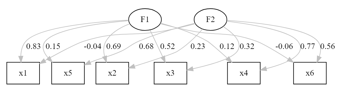
We have a fit with amazing indices, and loadings corresponding to the real model behind the data (remember that this is a simulated dataset). The only small concern is that x3 and x6 show loadings below .6 in their designated factors. Nonetheless, we have a CFA model that we could further tweak if we were doing the analysis in a completely exploratory perspective.
Final remarks
ESEM is a very powerful technique, but it is important to always compare it to regular CFA models if you have a clear a priori organization for your items (Marsh et al. 2014). Also, remember that having a good fit does not make a model correct! Always subject the results to theoretical scrutiny to check its validity.
References
Asparouhov, Tihomir, and Bengt Muthén. 2009. “Exploratory Structural Equation Modeling.” Structural Equation Modeling: A Multidisciplinary Journal 16 (3): 397–438. https://doi.org/10.1080/10705510903008204.
Marsh, Herbert W., Alexandre J. S. Morin, Philip D. Parker, and Gurvinder Kaur. 2014. “Exploratory Structural Equation Modeling: An Integration of the Best Features of Exploratory and Confirmatory Factor Analysis.” Annu. Rev. Clin. Psychol. 10 (1): 85–110. https://doi.org/10.1146/annurev-clinpsy-032813-153700.
Morin, Alexandre J. S., Herbert W. Marsh, and Benjamin Nagengast. 2013. “Exploratory Structural Equation Modeling.” In Structural Equation Modeling: A Second Course, 2nd Ed. Quantitative Methods in Education and the Behavioral Sciences: Issues, Research, and Teaching. IAP Information Age Publishing.
Revelle, William. 2020. Psych: Procedures for Psychological, Psychometric, and Personality Research. Northwestern University. https://CRAN.R-project.org/package=psych.
Rosseel, Yves. 2012. “lavaan: An R Package for Structural Equation Modeling.” Journal of Statistical Software 48 (2): 1–36. http://www.jstatsoft.org/v48/i02/.
Footnotes
In some recent work, authors have recommended the use of Target Rotations instead of the GeominQ. We use the GeominQ for simplicity, since Target Rotations require specifying a matrix of weights. This can also be accomplished with
psych.↩︎If you are more of a tidyverse user, just use
data.table::setDTto your tibble before inputing it in the function↩︎Part of my code for making the ESEM model is based on Tim Kaiser’s primer on ESEM, you can check it here↩︎